Tutorial (basic)

import numpy as np
import pandas as pd
from pytmle import PyTMLE

target_times = [5.0, 10.0, 15.0, 20.0, 25.0]
np.random.seed(42)

Load the Hodgkin’s Disease datase (adapted for Python from rfsrc):

df = pd.read_csv("hodgkins_disease.csv", index_col=0)
df

	female	extranod	stage2	medwidsi_S	medwidsi_N	chemo	time	status
age
64.00	1	0	0	0	1	0	3.1	2
63.00	0	0	0	0	1	0	15.9	2
17.00	0	0	1	0	1	0	0.9	1
63.00	0	0	1	0	1	0	13.1	2
21.00	0	0	1	0	0	0	35.9	0
...	...	...	...	...	...	...	...	...
23.24	1	0	1	1	0	0	6.2	0
43.00	1	1	1	0	0	1	12.0	0
44.05	1	0	1	0	0	1	14.9	0
53.99	1	0	0	1	0	0	12.3	0
28.49	0	0	1	0	0	1	12.3	0

865 rows × 8 columns

Instantiate the PyTMLE class according to the given dataset.

tmle = PyTMLE(df,
              col_event_times="time",
              col_event_indicator="status",
              col_group="chemo",
              target_times=target_times,
              g_comp=True,
              evalues_benchmark=True)

Fit PyTMLE with the stacking classifier for initial estimates of propensity scores and the state learner with default library for the hazards, using 5 CV folds, up to 100 TMLE updates and standard bootstrapping that uses all available cores. Set bootstrap=False to reduce execution time.

tmle.fit(cv_folds=5,
         max_updates=100,
         save_models=True,
         bootstrap=False,
         n_jobs=-1)

Estimating propensity scores...
Estimating hazards and event-free survival...
Estimating censoring survival...
Starting TMLE update loop...
TMLE converged at step 59.
Computing E-Value benchmark for female...

/home/jguski/COMMUTE/tmle/pytmle/pytmle/get_initial_estimates.py:377: RuntimeWarning: (DeepHit | CoxPHSurvivalAnalysis) failed: Matrix is singular.
  warnings.warn(

Computing E-Value benchmark for extranod...

/home/jguski/COMMUTE/tmle/pytmle/pytmle/get_initial_estimates.py:377: RuntimeWarning: (DeepHit | CoxPHSurvivalAnalysis) failed: Matrix is singular.
  warnings.warn(
/home/jguski/COMMUTE/tmle/pytmle/pytmle/evalues_benchmark.py:189: RuntimeWarning: Observed E-values are not defined for non-positive limiting bounds.
  warnings.warn(

Computing E-Value benchmark for stage2...

/home/jguski/COMMUTE/tmle/pytmle/pytmle/get_initial_estimates.py:377: RuntimeWarning: (DeepHit | CoxPHSurvivalAnalysis) failed: Matrix is singular.
  warnings.warn(

Computing E-Value benchmark for medwidsi_S...

/home/jguski/COMMUTE/tmle/pytmle/pytmle/get_initial_estimates.py:377: RuntimeWarning: (DeepHit | CoxPHSurvivalAnalysis) failed: Matrix is singular.
  warnings.warn(

Computing E-Value benchmark for medwidsi_N...

/home/jguski/COMMUTE/tmle/pytmle/pytmle/get_initial_estimates.py:377: RuntimeWarning: (DeepHit | CoxPHSurvivalAnalysis) failed: Matrix is singular.
  warnings.warn(

You can see in the warnings that some models do not converge, either because of non-singular matrices in Cox models or because the survival functions is estimated as 0 at some points. These model combinations are automatically discarded in the selection of the best model by the state learner.

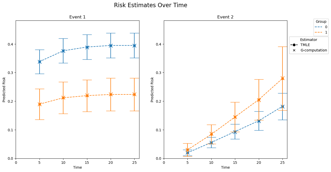
Plot the estimated CIF for both events. The ‘x’ markers show the effects that G-computation would yield without the TMLE update. If bootstrap=True was set in the fit method, you can also get bootstrapped quantile-based confidence intervals when setting use_bootstrap=True.

tmle.plot(g_comp=True, use_bootstrap=False)

(<Figure size 1400x700 with 2 Axes>,
 array([<Axes: title={'center': 'Event 1'}, xlabel='Time', ylabel='Predicted Risk'>,
        <Axes: title={'center': 'Event 2'}, xlabel='Time', ylabel='Predicted Risk'>],
       dtype=object))

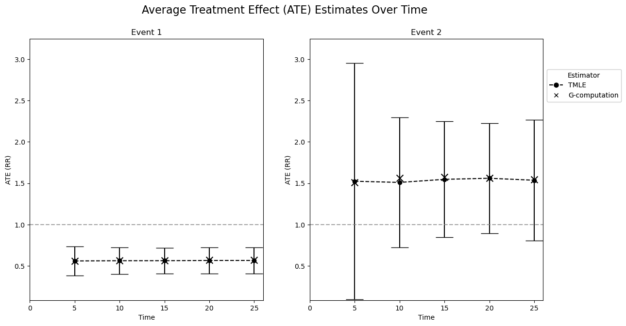
Plot the ATE estimates in terms of risk ratios. You can alternatively use type="rd" to use risk differences instead. If bootstrap=True was set in the fit method, you can also get bootstrapped quantile-based confidence intervals when setting use_bootstrap=True.

tmle.plot(g_comp=True, type="rr", use_bootstrap=False)

(<Figure size 1400x700 with 2 Axes>,
 array([<Axes: title={'center': 'Event 1'}, xlabel='Time', ylabel='ATE (RR)'>,
        <Axes: title={'center': 'Event 2'}, xlabel='Time', ylabel='ATE (RR)'>],
       dtype=object))

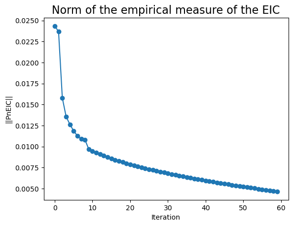
Plot \(||PnEIC||\) over TMLE iterations to check that it was minimized effectively.

tmle.plot_norm_pn_eic()

Plot the nuisance weights at baseline to check that positivity is not an issue. Set time=None to also get plots for baseline + all target times.

tmle.plot_nuisance_weights(time=0)

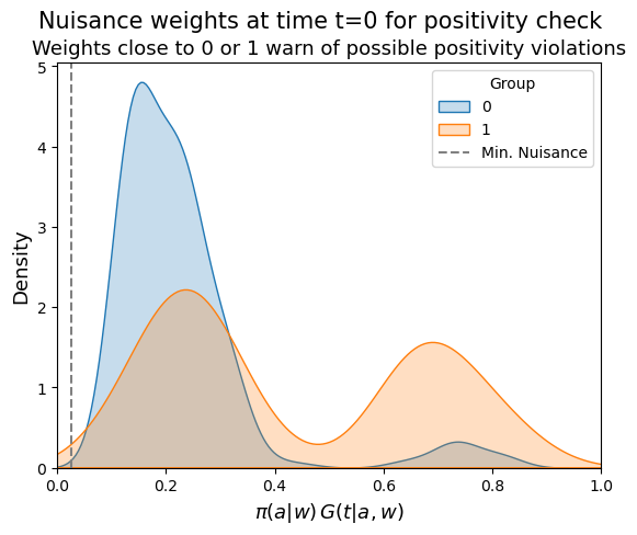
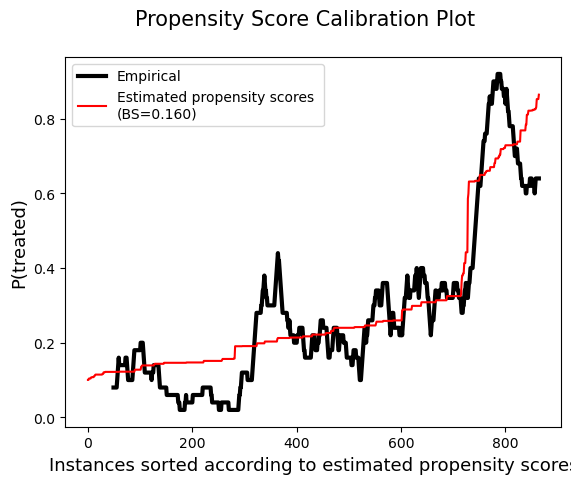
Propensity scores seem to be reasonably well calibrated.

tmle.plot_propensity_score_calibration()

Since save_models was set to True in the fit() call, you can extract the models used for initial estimates and analyze them further. In addition, you can inspect the loss for individual risks / censoring model combinations in the state learner.

print(tmle.models)
print(tmle.state_learner_cv_fit)

{'propensity_model': StackingClassifier(cv=5,
                   estimators=[('rf', RandomForestClassifier()),
                               ('gb', GradientBoostingClassifier())],
                   final_estimator=LogisticRegression(max_iter=1000)), 'risks_model_fold_0': CauseSpecificCoxPHSurvivalAnalysis, 'censoring_model_fold_0': CoxPHSurvivalAnalysis, 'risks_model_fold_1': CauseSpecificCoxPHSurvivalAnalysis, 'censoring_model_fold_1': CoxPHSurvivalAnalysis, 'risks_model_fold_2': CauseSpecificCoxPHSurvivalAnalysis, 'censoring_model_fold_2': CoxPHSurvivalAnalysis, 'risks_model_fold_3': CauseSpecificCoxPHSurvivalAnalysis, 'censoring_model_fold_3': CoxPHSurvivalAnalysis, 'risks_model_fold_4': CauseSpecificCoxPHSurvivalAnalysis, 'censoring_model_fold_4': CoxPHSurvivalAnalysis}
             risks_model        censoring_model      loss
4  CoxPHSurvivalAnalysis  CoxPHSurvivalAnalysis  3.099479
5  CoxPHSurvivalAnalysis   RandomSurvivalForest  3.110173
3  CoxPHSurvivalAnalysis                DeepHit  3.119103
7   RandomSurvivalForest  CoxPHSurvivalAnalysis  3.127392
6   RandomSurvivalForest                DeepHit  3.142220
8   RandomSurvivalForest   RandomSurvivalForest  3.142587
0                DeepHit                DeepHit  3.233718
1                DeepHit  CoxPHSurvivalAnalysis  3.248667
2                DeepHit   RandomSurvivalForest  3.272953

Plot the contours of the E-value for the effect estimates at a specific time for a specific event. If evalues_benchmark was set to True when initializing the PyTMLE class (as in this notebook), E-values for observed covariates are included. If bootstrap=True was set in the fit method, you can also get the E-values for bootstrapped confidence intervals when setting use_bootstrap=True.

tmle.plot_evalue_contours(time=25.0, event=1, type="rr", use_bootstrap=False)

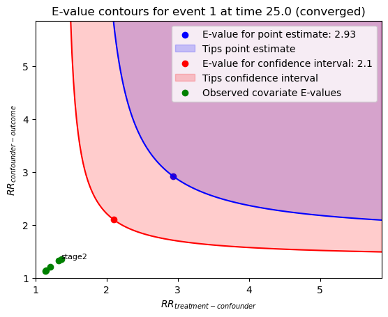
The E-values associated with the point estimate and CI for event 1 (relapse) at time 25 are clearly above the observed covariate E-values, which indicates that the treatment effect is rather robust.